Spotify With Machine Learning

Introduction

This fun project will use my personal Spotify music, along with my friend Kiran’s, with the goal to build several machine learning algorithms that will determine whose music library a song belongs to. I will explore several candidate models (k nearest neighbors, bagging, and random forest) to predict this binary outcome. To begin, the code to access your own Spotify account is included!

library(spotifyr)         # Spotify API interaction
library(here)             # Set file location
library(knitr)            # Creates nice tables
library(tidyverse)        # Data manipulation and visualization
library(tidymodels)       # Building machine learning models
library(rsample)          # Prepocessing datasets for machine learning
library(readr)            # Reads structured data files
library(dplyr)            # Data manipulation and transformation
library(ggplot2)          # Visualizations and plots
library(rpart)            # Decision tree algorithms
library(caret)            # Tools for machine learning models
library(rpart.plot)       # Visualization of decision trees
library(vip)              # Computes variable importance
library(pdp)              # Visualization of partial dependence plots
library(parsnip)          # Creating and tuning machine learning models
library(ipred)            # Bagging and bootstrapping for ensemble models
library(baguette)         # Building deep learning models

Access the Spotify API

To access the Spotify API, follow the link to Spotify For Developers (https://developer.spotify.com/) and follow these instructions:

• Select “Create a Client ID”

• Fill out form to create an app

• On dashboard page, click new app

• App’s dashboard page will have Client ID

• Click “Show Client Secret”

• Use the below code with your client ID and Client Secret in R!

Sys.setenv(SPOTIFY_CLIENT_ID = 'your_token')
Sys.setenv(SPOTIFY_CLIENT_SECRET = 'your_token')
 
access_token <- get_spotify_access_token(
   client_id = Sys.getenv("SPOTIFY_CLIENT_ID"),
   client_secret = Sys.getenv("SPOTIFY_CLIENT_SECRET")
)

I downloaded my liked songs, but the built-in function with the {spotifyr} package has a limit to download only 20 songs at a time. Below I wrote a loop to continue adding all of my liked songs into a dataframe.

songs_data <- data.frame()     # create base empty data frame
offset <- 0                    # starting point for spotify function offset
limit <- 20                    # maximum download at a time

while(TRUE) {                  # loop through all liked songs

  tracks <- get_my_saved_tracks(limit = limit, offset = offset)
  
  if(length(tracks) == 0) {    # setting when to stop the loop
    break
  }
  
  # add tracks into previously created dataframe
  songs_data <- rbind(songs_data, tracks)  
  
  offset <- offset + limit     # reset the loop to start at the next 20

}

There are other functions to play with inside this {spotifyr} package! I will not be exploring these further in this blog post.

bearicas_recent <- get_my_recently_played()
bearicas_top <- get_my_top_artists_or_tracks()
unique(bearicas_top$genres)

This initial data downloaded is not very exciting to play with. This data frame is mostly important to pull out the song ID column, and use that to connect back with Spotify’s API for downloading the specific audio features for each song. This function has a maximum download of 100 rows at a time so I created another loop below to download all the related audio features and bind the columns to the initial dataframe.

audio_features <- data.frame()        # create base empty data frame

for(i in seq(from = 1, to = nrow(songs_data), by = 100)) { 
  
  if (i > nrow(songs_data)) {         # setting when to stop the loop
    break
  }
  
  row_index <- i:(i + 99)             # collect 100 rows starting from i
  
  # pull out features for set rows
  audio <- get_track_audio_features(songs_data$track.id[row_index])
  
  # add features to dataframe
  audio_features <- rbind(audio_features, audio)
}

# will read in by 100, so may have NA's from the last loop
audio_features <- drop_na(audio_features)

# create data frame with songs and fun features!
ericas_audio <- cbind(audio_features, 
                      track.name = songs_data$track.name,
                      track.popularity = songs_data$track.popularity) |> 
  select(-c(uri, track_href, analysis_url, type))     # remove rows
  
# save as csv to share
write_csv(ericas_audio, "ericas_audio.csv")

My friend Kiran and I swapped data, which I will use to create a series of machine learning models to compare our music tastes. The goal is to create a model that can predict, using the audio features whose playlist it is from. I will go through four different types of models and at the end compare the metrics of each to decide which was most effective! The outcome variable will be the binary option of Kiran or Erica, set as listener_id.

ericas_audio <- ericas_audio |> 
  mutate(listener_id = "erica")

kirans_audio <- read_csv("kiran_audio.csv") |>  # get partner's data as csv
  mutate(listener_id = "kiran")

# combine datasets
total_audio <- rbind(ericas_audio, kirans_audio) |> 
  mutate(listener_id = as.factor(listener_id))
write_csv(total_audio, "total_audio.csv")

All of these previous steps culminate to this total_audio.csv file that I have previously saved and set aside, since I did not want to share my private Spotify information at the beginning.

total_audio <- read_csv(here("posts", "2023-02-22-spotify", "total_audio.csv")) |> 
    mutate(listener_id = as.factor(listener_id))

Data Exploration!

Code

total_audio %>%
  arrange(desc(instrumentalness)) |> 
  select(instrumentalness, track.name, track.popularity, listener_id) |> 
  rename('track name' = track.name,
         'track popularity' = track.popularity,
         'listener' = listener_id) |> 
  head(6) |> 
  kable()

instrumentalness	track name	track popularity	listener
0.971	Slow Blues - Instrumental	38	kiran
0.946	Orange	42	kiran
0.935	Ylang Ylang	61	kiran
0.924	Atlas	46	kiran
0.924	Defect	19	kiran
0.918	Master Tea	0	erica

Surprised to find out that the top instrumental songs belonged mostly to Kiran’s playlist, I mostly listen to music with strong drums and little lyrics so expected that I’d be in the top.

Code

total_audio %>%
  arrange(desc(acousticness)) |> 
  select(acousticness, track.name, track.popularity, listener_id) |> 
  rename('track name' = track.name,
         'track popularity' = track.popularity,
         'listener' = listener_id) |> 
  head(6) |> 
  kable()

acousticness	track name	track popularity	listener
0.994	Pachamama	58	erica
0.979	Flowers	57	erica
0.978	All We Do	56	erica
0.973	Whatever’s Written in Your Heart	29	kiran
0.942	The Forsaken Waltz	32	kiran
0.934	The View	8	erica

Although more of the top acoustic songs belonged in my playlist, Kiran listens to much louder music than me apparently.

Code

ggplot(total_audio, aes(x = track.popularity, y = listener_id)) +
  geom_boxplot(aes(fill = listener_id), color = "#000000", alpha = .8) +
  labs(title = "Distribution of Track Popularity by Listener",
       x = "Track Popularity", y = "Listener") +
  scale_fill_manual(values = c("#9954FE", "#289832")) +
  theme_minimal() +
  theme(plot.title = element_text(hjust = 0.5, face = "bold"),
        panel.grid.minor = element_blank(),
        panel.background = element_blank(),
        axis.line = element_line(colour = "black"),
        legend.position = "none")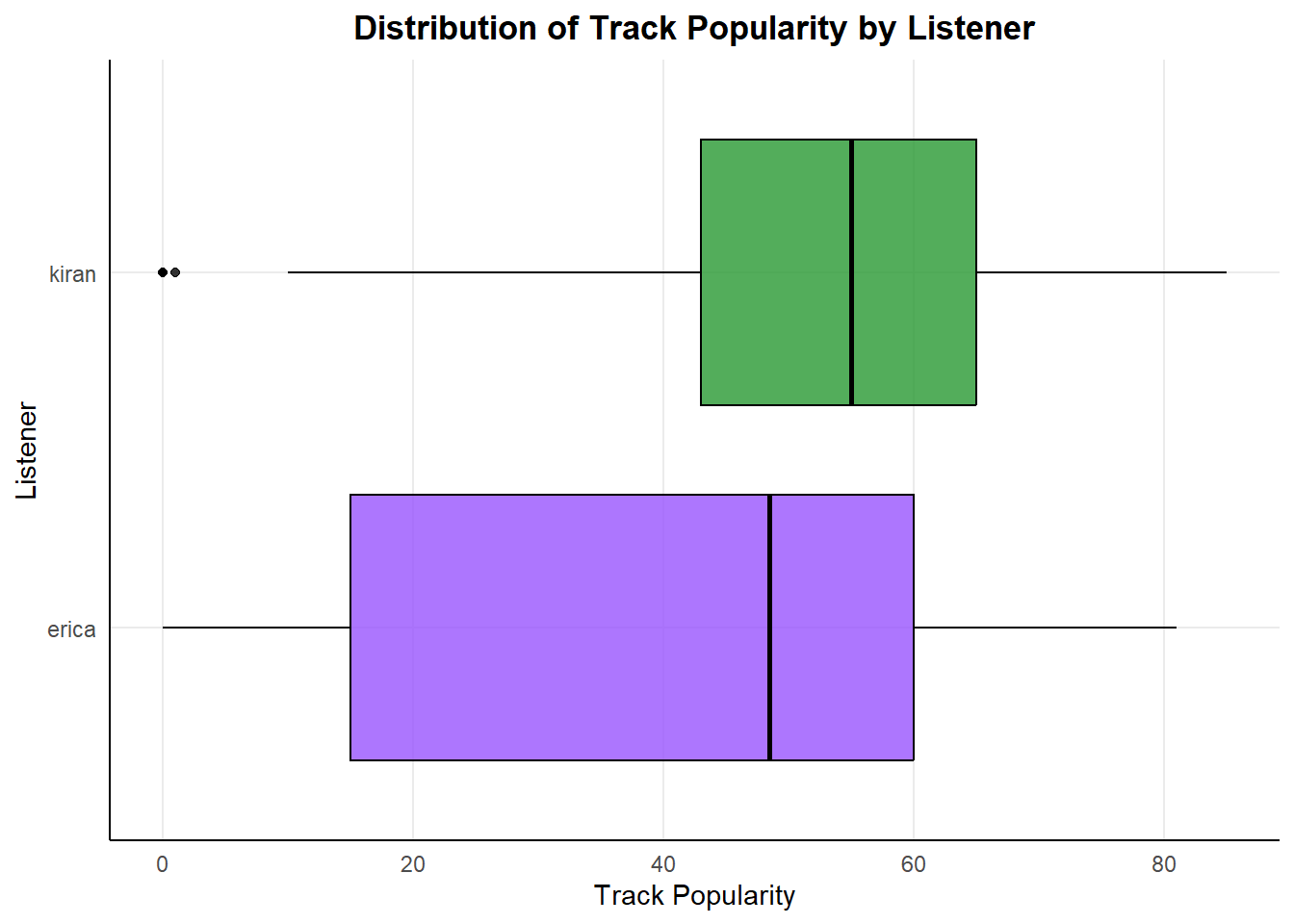

I listen to the most music listed as 0 popularity, so maybe I’m more underground and edgy with my style.

Code

ggplot(total_audio, aes(x = danceability, y = energy)) +
  geom_point(aes(color = listener_id), alpha = .8, size = 2) +
  labs(title = "Comparison of Dancing Styles",
       x = "Danceability", y = "Energy") +
  scale_color_manual(values = c("#9954FE", "#289832"),
                     labels = c("Erica", "Kiran")) +
  geom_text(x = .99, y = .97, label = "Party Dancing",
            color = "black", size = 4, hjust = 1, vjust = 1) +
  geom_text(x = 0.95, y = 0.2, label = "Slow Dancing",
            color = "black", size = 3.5, hjust = 1, vjust = 0) +
  geom_text(x = 0.2, y = 0.2, label = "Chill Zone",
            color = "black", size = 3.5, hjust = 0, vjust = 0) +
  theme_minimal() +
  theme(plot.title = element_text(hjust = 0.5, face = "bold"),
        panel.grid.minor = element_blank(),
        axis.line = element_line(colour = "black"),
        legend.position = "bottom")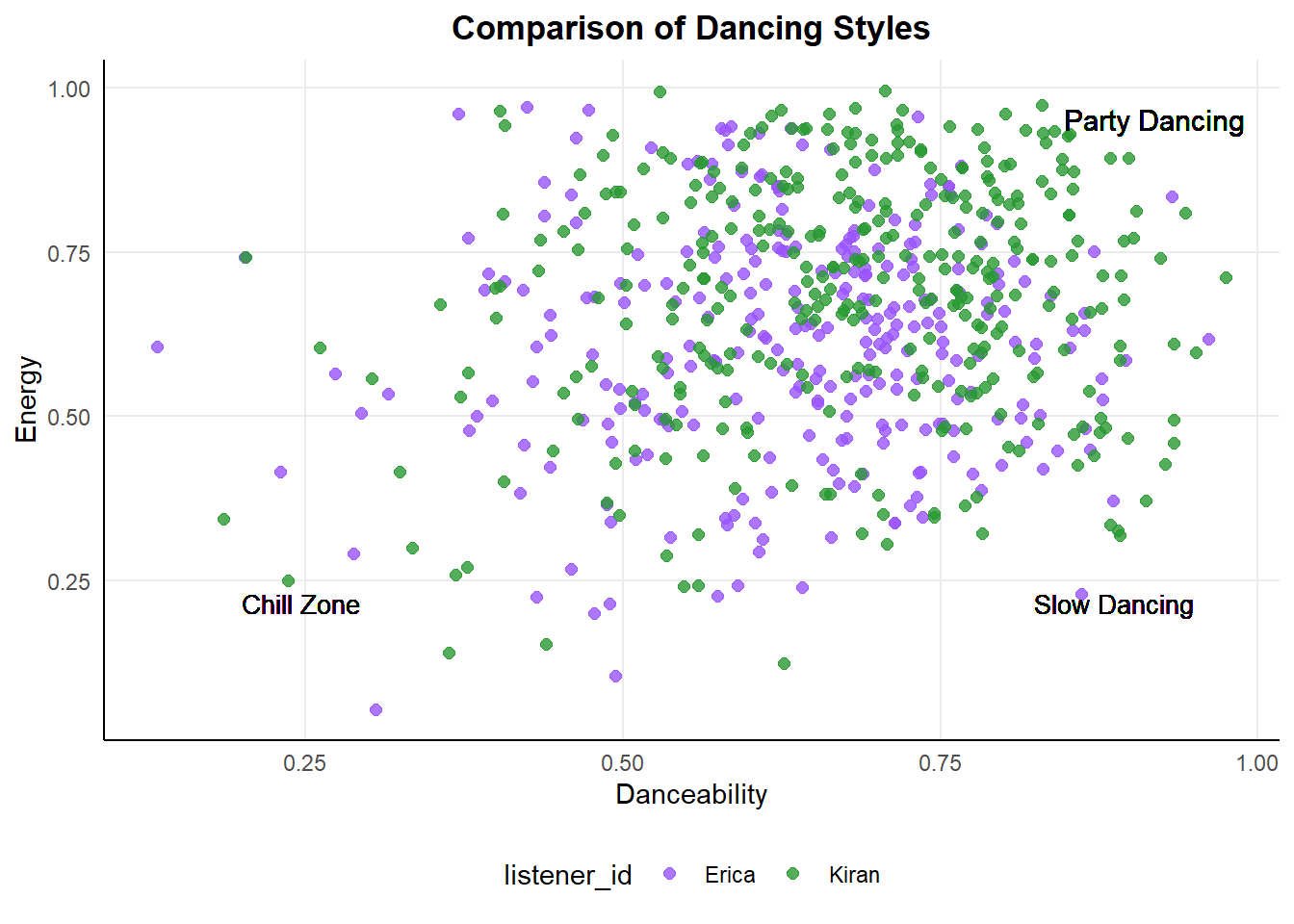

With this graph, low energy and high danceability would relate to slower (possibly romantic) songs, both of us appear to enjoy high energy and very danceable music but Kiran definitely goes harder.

Set Up Variables and Preprocessing

I will be creating several machine learning models, and use these variables as the start for them all. This initial train/test split is an important step to divide the dataset in two subsets. The training data will be used throughout to build each model. The test data will only be used once for each model at the end to evaluate the performance of the model on before unseen data. Keeping the data separated avoids leakage, which happens when the final testing data has influence the building of the model.

set.seed(61234)    # allows reproducibility

song_split <- initial_split(total_audio)
song_test <- testing(song_split) 
song_train <- training(song_split)

# Preprocessing, creating recipe with outcome and predictors
song_recipe <- recipe(listener_id ~ ., data = song_train) |> 
  
  # Keep data but do not use are predictor
  update_role(track.name, new_role = "ID") |>   
  update_role(id, new_role = "ID") |> 
  step_rm(track.name, id) |> 
  
  # Dummy code and normalize predictors
  step_dummy(all_nominal(), -all_outcomes(), one_hot = TRUE) |> 
  step_normalize(all_numeric(), -all_outcomes()) |> 
  
  prep()

# Cross Validation to tune parameter
cv_folds <- song_train |> 
  vfold_cv(v = 5)

K Nearest Neighbors Model

This is a type of supervised machine learning algorithm used for classification and regression tasks. In this case, I will be using it as classification because we have the binary output variable of listener_id. When predicting the value of an input data point, this model looks for the “K” closest data points within the training set. The output prediction is based on the majority class or mean value of the K neighbors.

set.seed(45634)

# Define nearest neighbor model
knn_spec <- nearest_neighbor(neighbors = 7) |> 
  set_engine("kknn") |> 
  set_mode("classification")

# Workflow
knn_workflow <- workflow() |> 
  add_model(knn_spec) |> 
  add_recipe(song_recipe)

# Fit resamples
knn_res <- knn_workflow |> 
  fit_resamples(
    resamples = cv_folds,
    control = control_resamples(save_pred = TRUE))

# Check Performance
knn_res |> collect_metrics()

# Tune the hyperparameters
knn_spec_tune <- nearest_neighbor(neighbors = tune()) |> 
  set_engine("kknn") |> 
  set_mode("classification")

# Workflow: Define new workflow
knn_workflow_tune <- workflow() |> 
  add_model(knn_spec_tune) |> 
  add_recipe(song_recipe)

# Fit workflow on predefined folds and hyperparameters
knn_cv_fit <- knn_workflow_tune |> 
  tune_grid(
    cv_folds,
    grid = data.frame(neighbors = c(1, 5, seq(10, 100, 10))))

# Check performance
knn_cv_fit |> collect_metrics()
# Results will show the n averaged over all the folds. Use this to predict the best.

# Workflow: Final
knn_final_wf <- knn_workflow_tune |> 
  finalize_workflow(select_best(knn_cv_fit, metric = "accuracy"))

# Fit: Final
knn_final_fit <- knn_final_wf |> fit(song_train)
knn_last_fit <- knn_final_wf |> last_fit(song_split)
knn_metrics <- knn_last_fit |> collect_metrics()

# Predict labels for test set
knn_pred <- predict(knn_final_fit,
                          new_data = song_test)

# Pull out actual listener
song_test_true <- song_test %>%
  select(listener_id)

# Evaluate model performance on test set
knn_perf <- knn_pred %>%
  bind_cols(song_test_true)

# View predicted and actual listeners
knn_perf |> 
  select(Predicted = .pred_class, Actual = listener_id) |> 
  slice(1:10) |> 
  kable()

Predicted	Actual
erica	erica
erica	erica
erica	erica
erica	erica
erica	erica
erica	erica
erica	erica
kiran	erica
erica	erica
erica	erica

knn_perf |> 
  metrics(truth = listener_id, estimate = .pred_class)

# A tibble: 2 x 3
  .metric  .estimator .estimate
  <chr>    <chr>          <dbl>
1 accuracy binary         0.692
2 kap      binary         0.378

Decision Tree

The next two models, bagging and random forests, use a series of decision trees. Decision tree models begin with all the data in a root node and making a split based on the most significant feature. Each split results in nodes of data to split on another feature, until there are finally no features left to split the data on. The model makes predictions by following the path from the root node to a leaf node following the rules set by each node split.

Bagging

Bagging is a form of bootstrap aggregation, this means that this is an ensemble model. The model constructs multiple versions of the same base model using random samples of the training data. All of these sub-models are aggregated into a final model. These steps improve the model performance by reducing variance and overfitting.

set.seed(4657345)

# Tune specs
tree_spec_tune <- bag_tree(
  mode = "classification",
  cost_complexity = tune(),
  tree_depth = tune(),
  min_n = tune()) |> 
  set_engine("rpart", times = 50)

# Define tree grid
tree_grid <- grid_regular(cost_complexity(), tree_depth(), min_n(), levels = 5)

# New workflow
wf_tree_tune <- workflow() |> 
  add_recipe(song_recipe) |> 
  add_model(tree_spec_tune)

# Build each model in parallel
doParallel::registerDoParallel()

# Fit model
tree_rs <- wf_tree_tune |>
  tune_grid(listener_id ~ .,
    resamples = cv_folds,
    grid = tree_grid,
    metrics = metric_set(accuracy))

# Final workflow
final_bag <- finalize_workflow(wf_tree_tune, select_best(tree_rs, "accuracy")) |> 
  fit(data = song_train)

# Predictions
bag_pred <- final_bag |> 
  predict(new_data = song_test) |> 
  bind_cols(song_test)

# Save metrics
bag_metrics <- bag_pred |> 
  metrics(truth = listener_id, estimate = .pred_class)

# View predicted and actual listeners
bag_pred |> 
  select(Predicted = .pred_class, Actual = listener_id) |> 
  slice(1:10) |> 
  kable()

Predicted	Actual
erica	erica
erica	erica
erica	erica
erica	erica
erica	erica
kiran	erica
erica	erica
kiran	erica
erica	erica
kiran	erica

# Evaluate performance
bag_pred |> 
  metrics(truth = listener_id, estimate = .pred_class)

# A tibble: 2 x 3
  .metric  .estimator .estimate
  <chr>    <chr>          <dbl>
1 accuracy binary         0.730
2 kap      binary         0.455

Random Forest

Random forest is another ensemble model, but this one cannot be done in parallel. This method creates multiple decision trees on random subsets of the data, and the key difference with this model is the random selection of features to include for each model. Not using all the features in each model then combining the decision trees improves the accuracy of the model.

# Define validating set
set.seed(1368)
val_set <- validation_split(song_train, 
                            strata = listener_id, 
                            prop = 0.70)

# Create Random Forest specification
rf_spec <-
  rand_forest(mtry = tune(),
              min_n = tune(),
              trees = 1000) %>%
  set_engine("ranger") %>%
  set_mode("classification")

# Define Random Forest workflow
rf_workflow <- workflow() %>%
  add_recipe(song_recipe) %>%
  add_model(rf_spec)

# Build in parallel
doParallel::registerDoParallel()
rf_res <- 
  rf_workflow %>% 
  tune_grid(val_set,
            grid = 25,
            control = control_grid(save_pred = TRUE),
            metrics = metric_set(accuracy))

# Output model metrics
rf_res %>% collect_metrics()

# Find the best accuracy metric
rf_res %>% 
  show_best(metric = "accuracy")

# Plot results
autoplot(rf_res) +
  theme_minimal()

# Select best Random Forest model
best_rf <- select_best(rf_res, "accuracy")

# Output predictions
rf_res %>% 
  collect_predictions()

# Defining final model while working in parallel
doParallel::registerDoParallel()
last_rf_model <- 
  rand_forest(mtry = 2, min_n = 3, trees = 1000) %>% 
  set_engine("ranger", importance = "impurity") %>% 
  set_mode("classification")

# Update workflow
last_rf_workflow <- 
  rf_workflow %>% 
  update_model(last_rf_model)

# Update model fit
rf_final_fit <- last_rf_workflow |> fit(song_train)

last_rf_fit <- 
  last_rf_workflow %>% 
  last_fit(song_split)

# Output model metrics
random_forest_metrics <- last_rf_fit %>% 
  collect_metrics()

# Predict on test set
rf_pred <- predict(rf_final_fit,
                     new_data = song_test) |> 
  bind_cols(song_test)

# Output the variables that are most important to our model
last_rf_fit %>% 
  extract_fit_parsnip() %>% 
  vip(num_features = 12) +
  ggtitle("Variable Importance Plot") +
  theme(plot.title = element_text(hjust = 0.5)) +
  theme_minimal()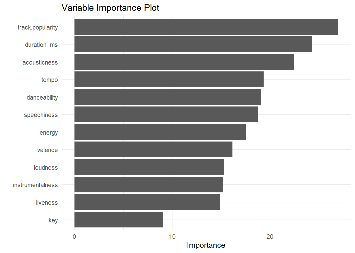

# View predicted and actual listeners
rf_pred |> 
  select(Predicted = .pred_class, Actual = listener_id) |> 
  slice(1:10) |> 
  kable()

Predicted	Actual
erica	erica
erica	erica
erica	erica
erica	erica
kiran	erica
erica	erica
erica	erica
kiran	erica
erica	erica
erica	erica

# Evaluate performance
rf_pred |> 
  metrics(truth = listener_id, estimate = .pred_class)

# A tibble: 2 x 3
  .metric  .estimator .estimate
  <chr>    <chr>          <dbl>
1 accuracy binary         0.730
2 kap      binary         0.453

Comparing Metrics

Code

# nearest neighbors metrics
knn_accuracy <- knn_metrics$.estimate[1]
 
# bag tree metrics
bag_accuracy <- bag_metrics$.estimate[1]

# Random Forest metrics
rf_accuracy <- random_forest_metrics$.estimate[1]


model_accuracy <- tribble(
  ~"model", ~"accuracy",
  "KNN", knn_accuracy,
  "Bagging", bag_accuracy,
  "Random Forest", rf_accuracy
)

ggplot(data = model_accuracy, aes(x = model, y = accuracy)) +
         geom_col(fill = "gray") +
  theme_minimal() +
  labs(title = "Comparison of Model Accuracy for Spotify Data",
       x = "Model", y = "Accuracy") +
  theme(plot.title = element_text(size = 16, face = "bold"),
        axis.title = element_text(size = 12),
        axis.text = element_text(size = 10)) +
  ylim(0,1)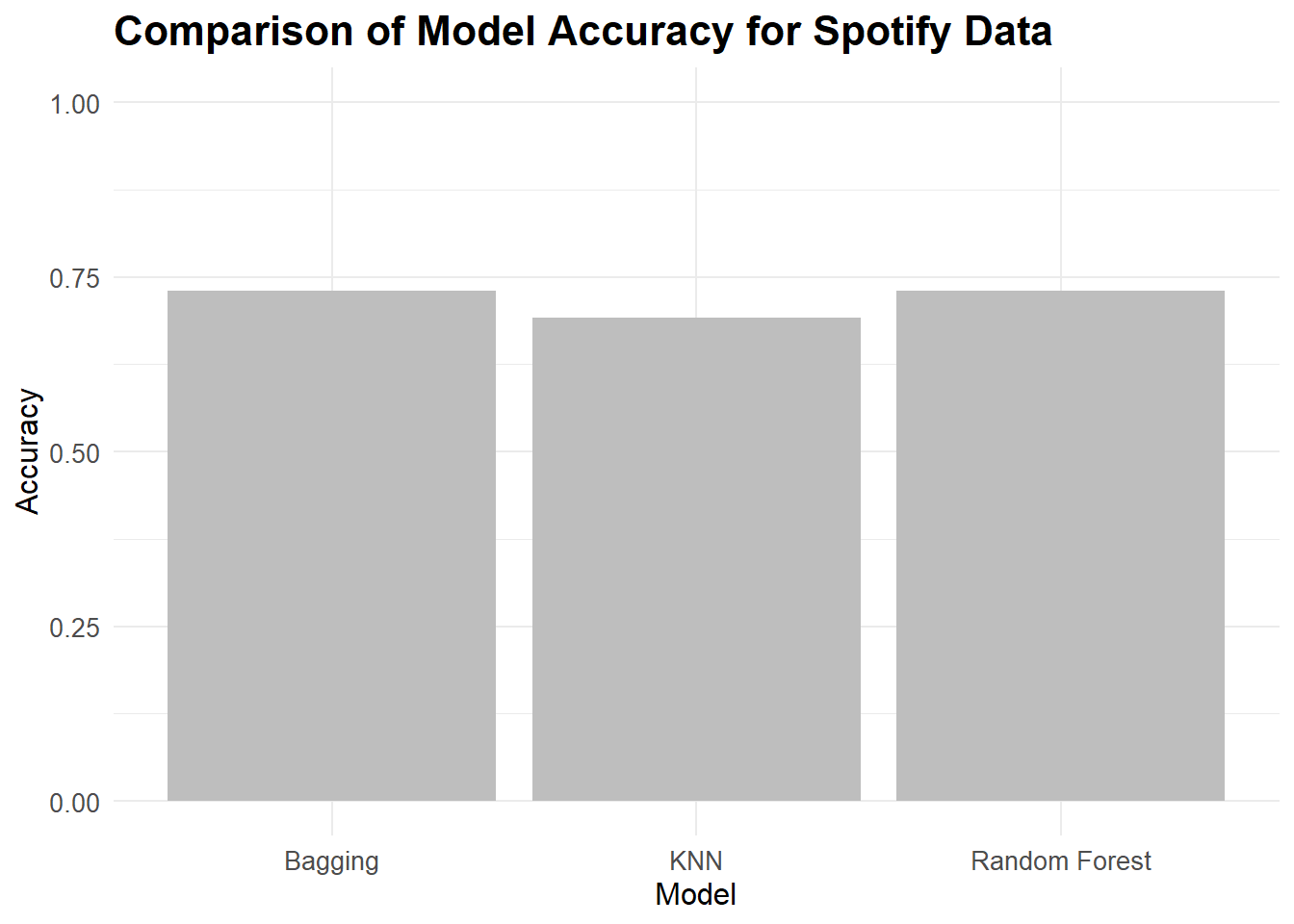

Citation

BibTeX citation:

@online{dale2022,
  author = {Dale, Erica},
  title = {Spotify {With} {Machine} {Learning}},
  date = {2022-12-09},
  url = {http://ericamarie9016.github.io/2023-02-22-spotify},
  langid = {en}
}

For attribution, please cite this work as:

Dale, Erica. 2022. “Spotify With Machine Learning.” December 9, 2022. http://ericamarie9016.github.io/2023-02-22-spotify.